13. NB. Linear Stability Analysis Using Orr-Sommerfeld Equation
Philipp Schlatter and Saleh Rezaeiravesh
pschlatt@mech.kth.se and salehr@kth.se
SimEx/FLOW, KTH Engineering Mechanics, Royal Institute of Technology, Stockholm, Sweden
This notebook is a part of the KTH-Nek5000 lecture notes.
#%matplotlib notebook
%matplotlib inline
import sys
import numpy as np
import scipy.linalg as scla
import matplotlib.pyplot as plt
from numpy.linalg import norm
import math as mt
pi=mt.pi
import matplotlib.pylab as pylab
sys.path.append('./')
from chebdif import chebdif      #chebdif function
params = {'legend.fontsize': 15,
          'legend.loc':'best',
          'figure.figsize': (8,6),
          'lines.markerfacecolor':'none',
          'axes.labelsize': 17,
          'axes.titlesize': 17,
          'xtick.labelsize':15,
          'ytick.labelsize':15,
          'grid.alpha':0.6}
pylab.rcParams.update(params)
13.1. Orr-Sommerfeld equation
In this notebook, the Orr-Sommerfeld equation is numerically solved for the laminar channel flow. The differentiations are approximated by the Chebyshev method which is discussed in a separate notebook.
The Orr-Sommerfeld equation for linear stability analysis can be derived as,
where \(\hat{v}=\hat{v}(y)\), \(U(y)\) is the velocity profile, \(Re\) denotes Reynolds number, \(\alpha\) is the wavenumber, and \(c\) is the phase speed. All derivatives are with respect to the spatial coordinates \(y\) where \(y\in[-1,1]\). Introducing the differentiation operator \(D\), where \(\hat{v}^{(n)} = D^n \hat{v}\) leads to,
which can be written as,
where \(\omega=c \alpha\). This equation defines a generalized eigenvalue problem.
13.2. Temporal stability analysis
For given \(Re\) and \(\alpha\), the Orr-Sommerfeld equation can be solved for the laminar channel flow with \(U(y)=1-y^2\). As a result, the eigenvalues \(c\in \mathbb{C}\) and associated eigenfunctions \(\hat{v}(y)\) are computed.
Set the solution settings:
Re = 5000    # Re_cl
alpha=1.12   # streamwise wavenumber
N=200        # resolution
Construct the differentiation operators:
The differential opertors are approximated by the Chebyshev method. As described in the Chebyshev notebook, we use a generalized formualtion of Chebyshev differentiation matrix as applied in chebdif.m, see Weideman and Reddy. A Python version of chebdif.m which is used here is taken from dmsuite, but small modifications have been applied.
The chebdif function called below is imported from chebdif.py.
y,D_=chebdif(N,1)
D=D_[0,:,:]
D2=D@D
D4=D2@D2
Construct the Orr-Sommerfeld operators A and B
# A*vhat = omega*B*vhat
I = np.identity(N)
A = -(D4-2*D2*alpha**2+I*alpha**4)/Re + 2j*alpha*I + 1j*alpha*np.diag(1-y**2)@(D2-I*alpha**2)
B = 1j*(D2-I*alpha**2)
Set the Boundary Conditions
# move the eigenvalues of the BC to Q
Q=-999j
# two homogeneous Dirichlet conditions
A[0,:] = Q*I[0,:]
B[0,:] = I[0,:]
A[-1,:] = Q*I[-1,:]
B[-1,:] = I[-1,:]
# two homogeneous Neumann conditions
A[1,:] = Q*D[0,:]
B[1,:] = D[0,:]
A[-2,:] = Q*D[-1,:]
B[-2,:] = D[-1,:]
Solve the eigenvalue problem
# compute eigenvalues and eigenvectors (A*vhat = omega*B*vhat)
omega,vv = scla.eig(A,B)
c=omega/alpha
Extract leading eigenvalue (TS wave)
i=np.argmax(c.imag)
cmax = c[i]

v=vv[:,i]
u=-np.dot(D,v)/(1j*alpha)  # use continuity equation i alpha u + Dv = 0

print('Leading eigenvalue c = ',cmax)
Leading eigenvalue c = (0.28175242719782523-0.0024847324977687536j)
Scale eigenvectors
i=np.argmax(abs(u))
w=u[i]
u/=w
v/=w
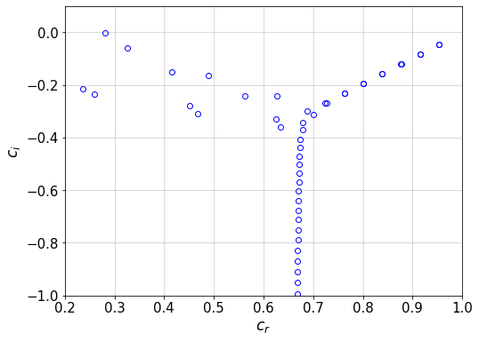
Plot the spectrum (eigenvalues)
#plt.figure()
plt.plot(c.real,c.imag,'ob')
plt.xlim([0.2,1])
plt.ylim([-1,0.1])
plt.grid()
plt.xlabel('$c_r$')
plt.ylabel('$c_i$')
plt.show()
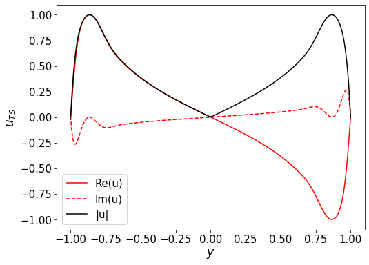
Plot amplitude of the perturbations
#plt.figure()
plt.plot(y,u.real,'r',label='Re(u)')
plt.plot(y,u.imag,'r--',label='Im(u)')
plt.plot(y,abs(u),'k-',label='|u|')
plt.legend(loc='best')
plt.xlabel(r'$y$')
plt.ylabel(r'$u_{TS}$')
plt.show()
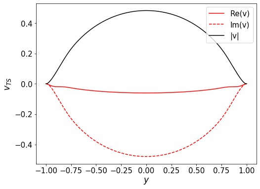
#plt.figure()
plt.plot(y,v.real,'r',label='Re(v)')
plt.plot(y,v.imag,'r--',label='Im(v)')
plt.plot(y,abs(v),'k-',label='|v|')
plt.xlabel(r'$y$')
plt.ylabel(r'$v_{TS}$')
plt.legend(loc='best')
plt.show()
13.3. Neutral stability curve for channel flow
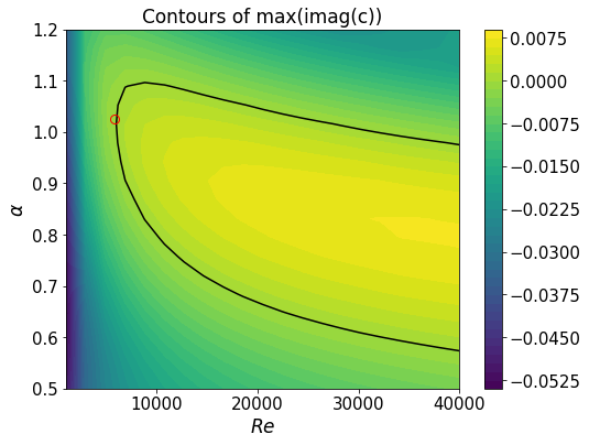
The aim is to compute the contours of the maximum \(imag(c)\) for given ranges of \(Re\) and \(\alpha\). Of particular interest is the isoline of \(max(imag(c))=0\) which specifies the neutral stability curve.
Create a mesh grid over the rectangular space of \(Re\times \alpha\)
N_Re=21
N_alpha=20
RE,ALPHA = np.meshgrid(np.linspace(1000,40000,N_Re),np.linspace(0.5,1.2,N_alpha))
Compute \(max(imag(c))\) for any \((Re,\alpha)\) in the mesh
g=np.zeros((N_Re,N_alpha))
for ii in range(N_Re):
    for jj in range(N_alpha):
        Re=RE[jj,ii]
        alpha=ALPHA[jj,ii]
        A = -(D4-2*D2*alpha**2+I*alpha**4)/Re + 2j*alpha*I + 1j*alpha*np.diag(1-y**2)@(D2-I*alpha**2)
        B = 1j*(D2-I*alpha**2)

        Q=-999j
        A[0,:] = Q*I[0,:]
        B[0,:] = I[0,:]
        A[-1,:]  = Q*I[-1,:]
        B[-1,:] = I[-1,:]
        A[1,:] = Q*D[0,:]
        B[1,:] = D[0,:]
        A[-2,:] = Q*D[-1,:]
        B[-2,:] = D[-1,:]

        omega,vv = scla.eig(A,B)
        g[ii,jj]=np.max(omega.imag)
Plot the contours
#plt.figure()
CS=plt.contourf(RE[0,:],ALPHA[:,0],g.T,levels=40)
plt.colorbar()
CS1=plt.contour(RE[0,:],ALPHA[:,0],g.T,levels=[0],colors='k')
plt.title('Contours of max(imag(c))')
plt.xlabel(r'$Re$')
plt.ylabel(r'$\alpha$')
plt.plot(5772,1.0255,'ro',ms=8) # Orszag 1971
plt.show()