1. Floating-point numbers
All numbers need to be stored in the computer’s memory. The main distinction is between integer and floating-point numbers, where integers are represented exactly (within in certain range), and floating-point numbers are approximated with an average relative error of \(\varepsilon_m\) called machine epsilon. The format of floating-point numbers is specified as IEEE norm 754, and supported on most (all) modern computers. The format to represent a number \(x\) is
where \(s\) is the sign, \(m\) the mantissa, \(b\) the base (typically 2) and \(e\) the exponent. The machine epsilon can now be calculated as \(\varepsilon_m=2^{-m}\). Depending on the required accuracy and speed, different standard formats are commonly used as summarised in the following table, see Fig. 1.1.
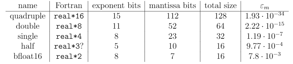
Fig. 1.1 Different IEEE floating-point formats according to norm 754.
1.1. Errors
The error of a numerical calculation is typically the combination of (at least) two errors, the truncation error \(\varepsilon_t\) and the round-off error \(\varepsilon_r\). The truncation error comes from the truncation of the Taylor series when approximating the derivative via finite differences, and is thus related to the order of the scheme. the round-off error, to the contrary, is related to the finite precision of the representation of numbers in a computer, for which the machine epsilon \(\varepsilon_m\) is a suitable quantification. Let us consider taking a derivative of a function, say
at \(x=2\) using central finite differences with spacing \(\Delta x\). Using double-precision arithmetics, the accuracy of the result is shown in Fig. 1.2.
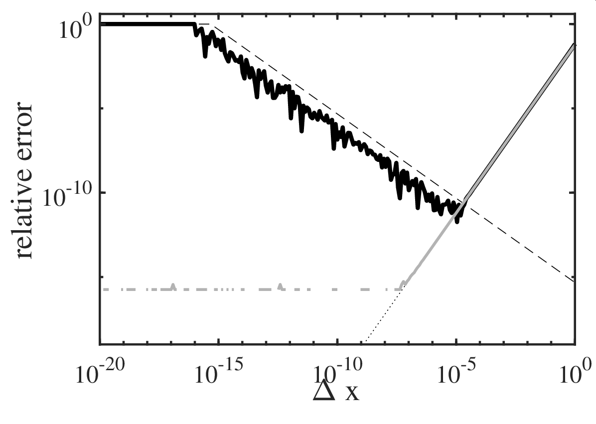
Fig. 1.2 Relative errror in the numerical computation of a derivative. (Solid black) central finite differences, (solid grey) complex-step method, (dashed) round-off error \(\varepsilon_r\), (dotted) truncation error \(\varepsilon_t\). Double-precision arithmetics with \(\varepsilon_m=2.22\cdot 10^{-15}\) is used.
Using Taylor series, the truncation error can estimated as
which shows that the method is indeed of second order. Considering the general formula for error propagation, the round-off error can be estimated as
It can be seen that the lowest error is not achieved for the smallest \(\Delta x\) due to cancellation (as quantified by the round-off error). An estimate for the optimal \(\Delta x\) can be obtained by considering the total error \(\varepsilon_t+\varepsilon_r\), and turns out to scale with \(\varepsilon_m^{1/3}\) for a second-order scheme (and \(\varepsilon_m^{1/2}\) for first-order one-sided finite differences). The knowledge of this behaviour is important in order to choose an appropriate step size \(\Delta x\) for general cases e.g. Newton–Krylov solvers).
1.2. Complex step method
Are there ways to avoid round-off errors? Realising that the problem comes from taking a difference of two numbers of nearly the same size, one could try to formulate a derivative without taking a difference. One such approach is the complex-step algorithm. Consider a Taylor expansion of \(f(x+i\Delta x)\) (instead of \(f(x+\Delta x)\) as for normal finite differences) with the complex unit \(i=\sqrt{-1}\). One then gets
A direct second-order accurate formula for \(f'(x)\) is thus
which does not involve differences, but complex arithmetic. Note that \(\mathrm{Im}\) denotes taking the imaginary part. As shown in Fig. 1.2, this formula indeed does not lead to round-off errors as the error for small \(\Delta x\) is close to \(\varepsilon_m\), and is second-order for larger \(\Delta x\). The complex-step algorithm is particularly useful in situations where very accurate approximations for derivatives of real functions are needed, e.g. in the evaluation of sensitivities using finite differences.
1.3. References
Press, W. H. and Teukolsky, S. A., Numerical calculation of derivatives, Computers in Physics 5, pp. 68, 1991.
Press, W. H., Teukolsky, S. A., Vetterling, W. T., and Flannery, B. P., Numerical Recipes: The Art of Scientific Computing, 3rd edition, Cambridge University Press, 2007.
Goldberg, D., What every computer scientist should know about floating-point arithmetic, ACM Computing Surveys, 23:1, 1991.