1. Spectral methods
1.1. Introduction
“Spectral methods” is a collective name for spatial discretisation methods that rely on an expansion of the flow solution as coefficients for ansatz functions. These ansatz functions usually have global support on the flow domain, and spatial derivatives are defined in terms of derivatives of these ansatz functions. The coefficients pertaining to the ansatz functions can be considered as a spectrum of the solution, which explains the name for the method.
Due to the global (or at least extended) nature of the ansatz functions, spectral methods are usually global methods, i.e. the value of a derivative at a certain point in space depends on the solution at all the other points in space, and not just the neighbouring grid points. Due to this fact, spectral methods usually have a very high order of approximation (spectral convergence meaning that the error with increasing resolution (number of grid points \(N\)) is in fact decreasing (faster than) exponentially (\(\varepsilon\propto (L/N)^{N}\)) as opposed to algebraically (\(\varepsilon\propto (L/N)^{p}\)) as for finite-difference methods). This behaviour is sketched in Fig. Fig. 1.3, where algebraic convergence means \(\log\varepsilon \propto -p\log N\) (straight line in log-log plot) and spectral convergence \(\log\varepsilon\propto -N\log N\) (“straight” line in lin-log plot).
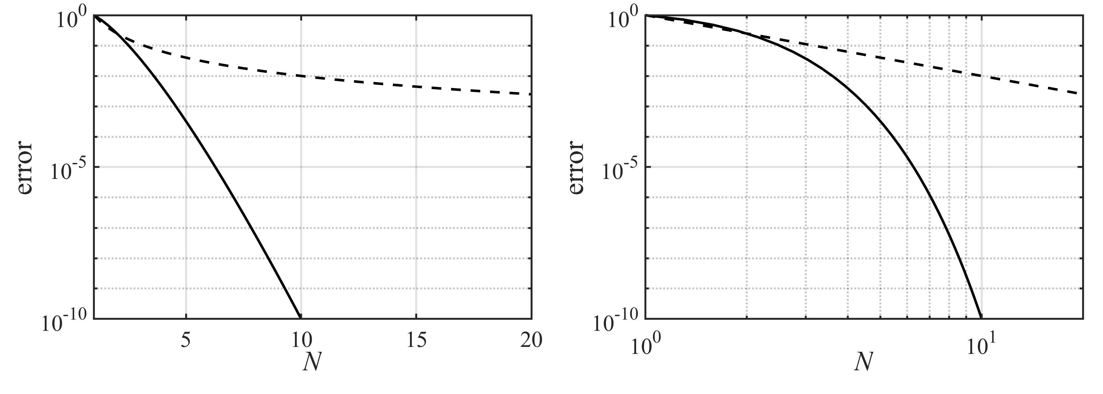
Fig. 1.3 Convergence behaviour of spectral convergence (solid, \(\varepsilon \propto (L/N)^{N}\)) and algebraic convergence (dashed, \(\varepsilon\propto (L/N)^{p}\)). The left panel is in log-lin scaling, and the right panel in log-log scaling.
In addition, dispersion and diffusion properties of the derivative operator are advantageous compared to finite-difference methods. This can be easily seen by considering the modified wave number concept: Spectral methods usually give the exact derivative of a function, the only error is due to the truncation to a finite set of ansatz functions/coefficients.
On the other hand, spectral methods are geometrically less flexible than lower-order methods, and they are usually more complicated to implement. Additionally, the spectral representation of the solution is difficult to combine with sharp gradients, e.g. problems involving shocks and discontinuitites. But for certain problems (mainly elliptic/parabolic problems in simple geometries) spectral methods are very adapted and efficient discretisation schemes.
In fact, spectral methods were among the first to be used in practical flow simulations. This was mainly prompted due to their high order of accuracy, meaning that an accurate solution could already be represented with a lower number of grid points. This cautious use of (expensive) computer memory was essential in the early days of CFD. In this regard, consider for instance the two seminal papers using spectral methods:
Stability analysis of a channel flow by S. A. Orszag (1971) “Accurate solution of the Orr-Sommerfeld stability equation”, Journal of Fluid Mechanics, Vol. 50, pp. 689-703. In this paper the critical Reynolds number for channel flow, i.e. \(Re=5772\) was computed using a Chebyshev-tau method.
The first direct numerical simulation (DNS) of a channel flow at \(Re_\tau=180\) by J. Kim, P. Moin and R. Moser (1987) “Turbulence statistics in fully developed channel flow at low Reynolds number”, Journal of Fluid Mechanics, Vol. 177, pp. 133-166.
The topic of spectral methods is very wide, and various methods and sub-methods have been proposed and are actively used. The following description aims at giving the fundamental ideas, focusing on the popular Chebyshev-collocation and Fourier–Galerkin methods.
1.2. General references
C. Canuto, M. Hussaini, A. Quarteroni and T. Zang. Spectral Methods. Fundamentals in Single Domains. Springer Verlag, 2006.
C. Canuto, M. Hussaini, A. Quarteroni and T. Zang. Spectral Methods. Evolution to Complex Geometries and Applications to Fluid Dynamics. Springer Verlag, 2007.
J. P. Boyd. Chebyshev and Fourier Spectral Methods. 2000. Online http://www-personal.umich.edu/~jpboyd/BOOK_Spectral2000.html. Specifically for Chebyshev methods:
L. N. Trefethen, Spectral Methods in MATLAB, SIAM, Philadelphia, 2000. Homepage: https://people.maths.ox.ac.uk/trefethen/spectral.html
J. A. C. Weideman and S. C. Reddy. A MATLAB differentiation matrix suite. ACM Transactions of Mathematical Software, Vol. 26, pp.\ 465-519, 2000. Download the code at http://dip.sun.ac.za/~weideman/research/differ.html.