3. Fourier series
Fourier series are particularly suited for the discretisation of periodic functions \(u(x) = u(x+L)\) (Joseph Fourier 1768–1830). For such a periodic domain with periodicity \(L\), we define the fundamental wave number \(\alpha=2\pi/L\), and the Fourier functions are
with integer wave numbers \(k\). The \(2K+1\) coefficients \(c_k\) are the complex Fourier coefficients for the Fourier mode \(\Phi_k(x)=\exp(\mathrm{i}\alpha kx)\), as illustrated in Fig. 3.1. Note that the summation limits are sometimes also denoted as \(|k|\leq N/2\) with \(N=2K\). Additionally, a Fourier-transformed quantity is often denoted by a hat, \(\hat{u}_k = c_k\).
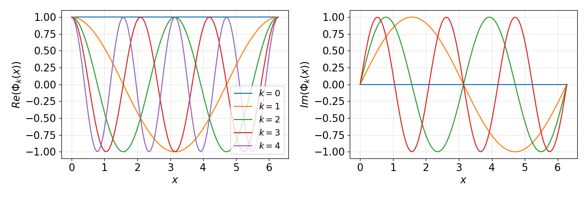
Fig. 3.1 Fourier functions \(\Phi_k(x)=\exp( \mathrm{i}\alpha kx)\) for \(k=0,\ldots,3\) with \(\alpha=2\pi/L=1\). The wave number \(k\) describes how many waves fit into the domain \(L\).
A Fourier series of a smooth function (also in the derivatives, i.e. part of \(C_\infty\)) converges rapidly with increasing \(N\), since the magnitude of the coefficients \(|c_k|\) decreases exponentially. This behaviour is called spectral convergence. However, if the original function \(u(x)\) is non-continuous in at least one of the derivatives \(u^{(p)}(x)\), the rate of convergence is severely decreased to order \(p\), i.e.
which corresponds to algebraic convergence as for finite-difference methods. It is thus very important that Fourier methods are only efficient for smooth functions.
This phenomenon is usually referred to as the Gibbs phenomenon (Josiah Willard Gibbs 1839–1903), according to which spurious oscillations can be seen in the interpolant around sharp gradients. This behaviour is shown in Fig. 3.2 for a top-hat function featuring a discontinuity in the function itself, i.e. in \(u^{(0)}\). Then, the order of convergence of the series expansion (2.2) is limited to zeroth order \(p=0\), i.e. the error does not decrease further with refinement of the grid.
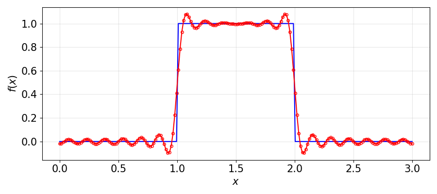
Fig. 3.2 Illustration of the Gibbs phenomenon: Fourier interpolation of a function with sharp gradients leads to spurious oscillations near the discontinuity. Note that the amplitude of the wiggles does not further decrease with higher resolution.
The transformation from the space of the discrete representation of \(u_N\) (physical space) to the space of the Fourier components \(c_k\) (spectral space) is called the (forward) discrete Fourier transform \(\mathcal{F}(u_N)\). Correspondigly, the reverse transform is the inverse Fourier transform \(\mathcal{F}^{-1}(c_k)\). An efficient way to compute this is via the fast Fourier transform (FFT) (Cooley and Tukey 1965 going back to an idea by Carl Friedrich Gauss 1805), thereby reducing the computational effort from \(\mathcal{O}(N^2)\) to \(\mathcal{O}(N\log(N))\) in one dimension. Note that there are various definitions of the scalings of the Fourier coefficients and the transforms, see the notebook NB. Fourier Transform. Perhaps the most used library for FFTs these days is FFTW (fastest Fourier transform in the West) which performs well on various architectures due to their adaptive algorithm.
Other important properties of Fourier series are:
Orthogonality:
with the Kronecker symbol \(\delta_{kl}\) and the complex conjugate \(\Phi_l^*(x)\).
Product rule:
Differentiation:
Discrete transforms \(u_N(x_j)\leftrightarrow c_k\): Based on the discrete orthogonality relation (\(N=2K+1\); \(|k|,|m|\leq K\))
the relation between physical and spectral space is shown in a straight-forward way to be
Note that we have restricted \(|k|,|m|\leq K\) so that aliasing errors are not present here, as opposed to further down. These relations can be used to transform between the physical and spectral space, and are called a ``discrete Fourier transform’’ (implemented e.g. using FFT). As any linear relation, the Fourier transform can be viewed as a matrix–vector multiplication with a full matrix composed of \(\Phi_k(x_j)\).
Some of the aspects are demonstrated in the attached notebooks. In particular, the notebook NB. Fourier wavenumbers discusses the peculiarities of real-to-complex transforms typically appearing in CFD applications, and general aspects of Fourier transforms are discussed in NB. Fourier Transform.