8. NB Numerical accuracy
Philipp Schlatter
pschlatt@mech.kth.se
SimEx/FLOW, KTH Engineering Mechanics, Royal Institute of Technology, Stockholm, Sweden
This notebook is a part of the KTH-Nek5000 lecture notes.
import numpy as np
from math import pi
from numpy.linalg import norm
import matplotlib.pyplot as plt
import matplotlib.pylab as pylab
params = {'legend.fontsize': 15,
          'legend.loc':'best',
          'figure.figsize': (14,5),
          'lines.markerfacecolor':'none',
         'axes.labelsize': 17,
         'axes.titlesize': 17,
         'xtick.labelsize':15,
         'ytick.labelsize':15,
         'grid.alpha':0.6}
pylab.rcParams.update(params)
#%matplotlib notebook
%matplotlib inline
8.1. Machine epsilon
Three different ways to compute the machine epsilon \(\varepsilon_m\):
# using the typical algorithm: divide by two until there is no difference any longer
def machineEpsilon(func=float):
    machine_epsilon = func(1)
    while func(1)+func(machine_epsilon) != func(1):
        machine_epsilon_last = machine_epsilon
        machine_epsilon = func(machine_epsilon) / func(2)
    return machine_epsilon_last
machineEpsilon(float)
2.220446049250313e-16
# using finfo
np.finfo(float).eps
2.220446049250313e-16
# using the definition of the bit size of the mantissa (for float nmant=52)
2**-np.finfo(float).nmant, 2**-52
(2.220446049250313e-16, 2.220446049250313e-16)
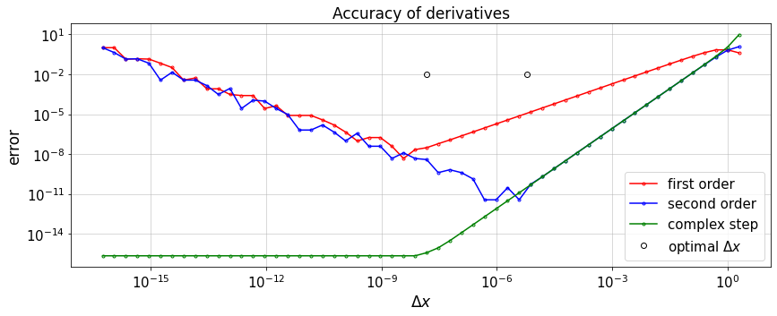
8.2. Accuracy of derivatives
Compare different types of errors in the computation of derivatives (truncation error and round-off error).
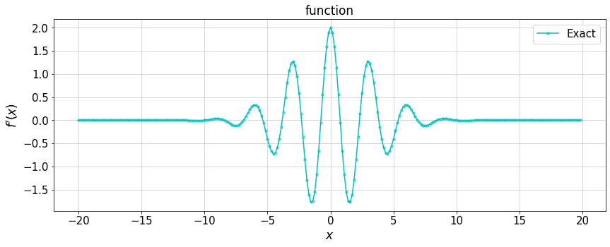
# Analytical f(x) and f'(x)
f = lambda  x: np.sin(2*x)*np.exp(-x**2/20)
fp = lambda x: 2*np.cos(2*x)*np.exp(-x**2/20)-(2/20)*x*f(x)
i=8
L=40
n=int(2**i)

#create data
dx=L/n
x=np.linspace(-L/2,L/2-dx,n)


fx=f(x)
fpx=fp(x)

#plot
plt.figure(figsize=(14,5))
plt.title('function')
plt.plot(x,fpx,'.-c',label='Exact')
plt.xlabel(r'$x$')
plt.ylabel(r'$f^\prime(x)$')
plt.grid()
plt.legend(loc='upper right')
plt.show()
x=1.
DX=[]
E1=[]
E2=[]
E3=[]
for i in range(-54,2):
   dx = 2**i

   df1 = (f(x+dx)-f(x))/dx
   e1 = abs(df1-fp(x))/abs(fp(x))
   E1.append(e1)

   df2 = (f(x+dx)-f(x-dx))/2/dx
   e2 = abs(df2-fp(x))/abs(fp(x))
   E2.append(e2)

   df3 = np.imag(f(x+1j*dx))/dx
   e3 = abs(df3-fp(x))/abs(fp(x))
   e3 = max (e3,np.finfo(float).eps)
   E3.append(e3)

   DX.append(dx)

#plot
plt.figure(figsize=(14,5))
plt.title('Accuracy of derivatives')
plt.loglog(DX,E1,'.-r',label='first order')
plt.loglog(DX,E2,'.-b',label='second order')
plt.loglog(DX,E3,'.-g',label='complex step')
plt.plot((2**-52)**(1/2),0.01,'ok',label="optimal $\Delta x$")
plt.plot((2**-52)**(1/3),0.01,'ok')
plt.xlabel('$\Delta x$')
plt.ylabel('error')
plt.grid()
plt.legend(loc='lower right')
plt.show()