.md .pdf

4. Chebyshev polynomials

As stated, Fourier series are only a good choice for periodic function. For problems with non-periodic boundary conditions, ansatz functions based on orthogonal polynomials are preferred. One popular choice are the Chebyshev polynomials (Pafnuty Lvovich Chebyshev, 1821–1894), defined on a domain $x\leq|1|$ as

$$\begin{equation} T_k(x) = \cos(k \arccos x) \ , \ \ k=0, 1, 2, \ldots \ . \end{equation}$$

The first polynomials are thus (see also Fig. 4.1)

$$\begin{split} \begin{eqnarray} T_0(x) &=& 1 \\ T_1(x) &=& x \\ T_2(x) &=& 2x^2 -1 \\ T_3(x) &=& 4x^3-3x \ . \end{eqnarray} \end{split}$$

There exists also a recursion formula

$$\begin{equation} T_{k+1}(x) + T_{k-1}(x) = 2 x T_k(x) \ , \ \ k\geq 1 \ . \end{equation}$$

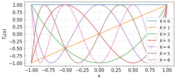
Fig. 4.1 Chebyshev polynomials $T_k(x)$ for $k=0,\ldots,6$.

A function $u(x)$ is approximated via a finite series of Chebyshev polynomials as

(4.1) $$\begin{equation} u_N(x) = \sum_{k=0}^N a_k T_k(x) \ , \end{equation}$$

with the $a_k$ being the Chebyshev coefficients. Note that the sum goes from 0 to $N$, i.e. there are $N+1$ coefficients. The highest order of the polynomial approximation is thus $N$.

A general problem of high-order interpolation of a function via high-order polynomials is the Runge phenomenon (Carl David Tolmé Runge 1856–1927), similar to the Gibbs phenomenon for Fourier series. If a function is interpolated on an equidistant grid, the error grows as $2^N$. However, using a non-equidistant distribution of points such that the point density is (approximately) proportional to $N \sqrt{1-x^2}^{-1}$, i.e. denser towards the domain boundaries, it can be shown that the interpolation errors decrease exponentially.

A common distribution of points in particular for Chebyshev polynomials are the Gauss–Lobatto–Chebyshev (GLC) points

(4.2) $$\begin{equation} x_j = \cos \frac{\pi j}{N} \ , \ \ j=0,\ldots,N \ . \end{equation}$$

The $N+1$ points $x_j$ correspond to the locations of the extrema of $T_N=\pm 1$. A more intuitive way of visualising the GLC nodes is by diving a half circle into $N$ identical sectors and projecting their edge coordinates.

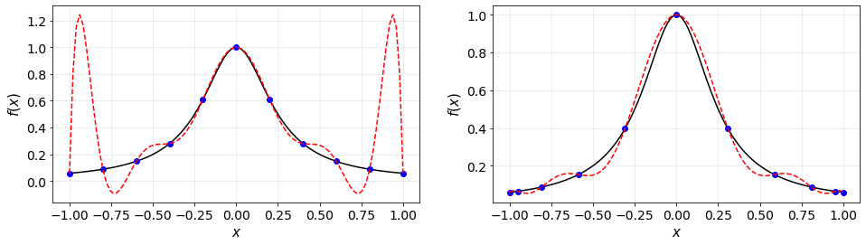
Fig. 4.2 Illustration of the Runge phenomenon: Polynomial interpolation of the function $f(x) = (1+16x^2)^{-1}$ on equidistant and non-equidistant (Gauss–Lobatto–Chebyshev) grids.

Chebyshev polynomials have a number of important properties:

• Alternating even and odd functions:

$$T_k(-x) = (-1)^k T_k(x) \ .$$

• Orthogonality (note the weight in the inner product):

$$\begin{equation} (T_k,T_l) = \int_{-1}^1 \frac{T_k(x) T_l(x)}{\sqrt{1-x^2}}\mathrm{d}x = \frac{\pi}{2} c_k \delta_{kl} \ , \end{equation}$$

with $c_0=2$, $c_k=1$ for $k\geq1$ and the Kronecker symbol $\delta_{kl}$.

• Boundary conditions:

$$\begin{equation} T_k(1) = 1 \text{ and } T_k(-1) = (-1)^k \ . \end{equation}$$

• To evaluate the finite Chebyshev series (4.1) use the stable recursive algorithm

$$\begin{split} \begin{eqnarray} B_{N+1} &=& 0 \ , \ \ B_N = a_N \nonumber\\ B_k &=& a_k +2xB_{k+1} -B_{k+2} \ , \ \ k=N-1,\ldots,1\nonumber\\ u_N(x) &=& a_0 -B_2 + B_1 x\nonumber \ . \end{eqnarray} \end{split}$$

• The values of the Chebyshev polynomials on the Gauss-Lobatto nodes are

$$\begin{equation} T_k(x_j) = \cos\left( \frac{k j \pi}{N} \right)\ , \ \ j,k=0,\ldots,N\nonumber \end{equation}$$

The transformation between the physical space $u_N$ and spectral (Chebyshev) space $a_k$ is done via the so-called Chebyshev transform. Since the Chebyshev polynomials are essentially cosine functions on a transformed coordinate, there exists a fast transform based on the FFT. As usual, the linear transform can also be represented by a matrix–vector multiplication with a full matrix.

If a collocation method on the Gauss-Lobatto grid (4.2) is employed, the derivative of a discretised function $u_N$ can be written as a matrix multiplication,

$$\begin{equation} u_N' (x_i) = \sum_{j=0}^N D_{ij} u_N (x_j) \ . \end{equation}$$

The matrix $\underline{\underline{D}}=[D_{ij}]$ is known as the (Chebyshev) derivative matrix, and represents a transformation into spectral space, spectral derivation and back-transform. An explicit form of the $(N+1)\times(N+1)$-matrix $\underline{\underline{D}}=[D_{ij}]$ is given by

$$\begin{split} \begin{equation} D_{ij} = \left\{\begin{array}{cc} \frac{c_i}{c_j} \frac{(-1)^{i+j}}{x_i-x_j} \ , & i\neq j \\ - \frac{x_i}{2(1-x_i^2)} \ , & 1\leq i=j \leq N-1 \\ \frac{2 N^2+1}{6} \ , & i=j=0 \\ -\frac{2N^2+1}{6} \ , & i=j=N \ , \end{array} \right. \end{equation} \end{split}$$

with

$$\begin{split} \begin{equation} c_{k} = \left\{\begin{array}{cc} 2 \ , & k=0, N \\ 1 \ , & 1\leq k \leq N-1 \ . \end{array} \right. \end{equation} \end{split}$$

Note that the computation of $\underline{\underline{D}}$ is very sensitive to round-off errors. Therefore, it is recommended for practical computations to use specificially adapted versions of the above formula, e.g. chebdif.m from “A Matlab Differentiation Matrix Suite” by J.A.C. Weideman and S.C. Reddy (or the corresponding Python versions as in the attached notebooks.

3. Fourier series 5. Linear stationary case